HE Convolution Theorem
Definitions:
- Let d = the incoming dyad that we're measuring
- Let i signify one of the "basis" JI intervals
- Let
= entropy
- Let
= a normalized Gaussian curve of standard deviation s and mean m evaluated at point d -
- Let
= the integral of the above: a cumulative distribution function of standard deviation s and mean m evaluated at point d -
- Let
= a rectangle function of lower bound l and upper bound u, evaluated at point d. this = 1 iff l <= d <= u, 0 otherwise
-
= the lower bound for the domain for some interval i
-
= the upper bound for the domain for some interval i
- Let
= the rectangle function for interval i, which is centered at i and has a width of some constant k times 1//sqrt(n*d), evaluated at point d
- Let
= the probability that d is heard as some interval i
- Let
= The convolution of f(x) and g(x), taken at x.
Approach:
To begin, let's look at the HE equation:
We will thus start by recomputing
Proof:
From HE:-
Defined as part of the HE equation[1]
-
This is the actual integral computed out algebraically
-
However, going back to (1), instead of taking the definite integral from point a to b, we can multiply the function pointwise by a rect function that is 1 between a and b, and 0 otherwise, and take the indefinite integral. They're the same thing.
-
Since a Gaussian curve is symmetric about the x-axis
-
(4) with (3)
-
This is equivalent to convolution, by definition #11
-
HE definition
-
By substituting (5) in for the
-
-
-
-
Let
be the Kroenecker delta function, which is 1 at d=0 and 0 otherwise
-
We can factor the Gaussian term out, since convolution is associative with scalar multiplication and distributive over addition; we approximate the log term by a constant scalar function
-
As the number of intervals increases, the log term approaches an infinite yet scalar value
-
As the rect function turns into a Kroenecker delta, and as the logarithm tends towards infinity, we approach a scaled Dirac delta, weighted by some interval-specific constant k_i
-
(15) with (14)
-
Definition
-
(16) with (17)
-
The Dirac delta acts as an identity operator for convolution; convolution with a scaled Dirac delta yields a scaled version of the original function, and convolution with a time-shifted Dirac delta yields a time-shifted version of the original function
Now let's get the entropy:
Now, HE is usually computed over some finite series that, if left to run, would enumerate the rationals. The most common
one is the Tenney series, in which all rationals of the form n/d are included provided n*d is less than some cutoff N. As
more intervals are added, we note that:
As N tends to infinity, %20-%20C_s(i_l%20-%20d))) tends to
become closer and closer to a constant function approaching a scalar value. In light of this, we can use the following
approximation, which converges to an exact equivalence as the number of intervals in the series tends towards infinity:
tends to
become closer and closer to a constant function approaching a scalar value. In light of this, we can use the following
approximation, which converges to an exact equivalence as the number of intervals in the series tends towards infinity:
Therefore:
Let's simplify this by turning the entire summation on the right into a convolution kernel function K(d):
Thus, Harmonic Entropy can be represented as the convolution of a Gaussian curve and a "basis" function K(d). QED.
The following is also true:This also proves that, although HE was originally conceptualized as a model whereby the incoming dyad is spread out with an error function, it can also be viewed as a model whereby the incoming dyad remains pure and the basis JI intervals are the ones that get spread out with an error function.
Previous attempts of mine to emulate the HE algorithm with a convolution set it up so that each JI interval is dispersed uniformly with a Gaussian error function; HE is however set up such that each JI interval gets its own spreading function as well as the general spreading function of the Gaussian. It remains to be proven whether or not the two converge as the number of rationals used as basis intervals tends to infinity. What exactly this means will become apparent shortly.
So what exactly IS K(x)? What does the convolution kernel for HE look like? Here's a picture of the kernel for n*d<10000, s=1.2%:
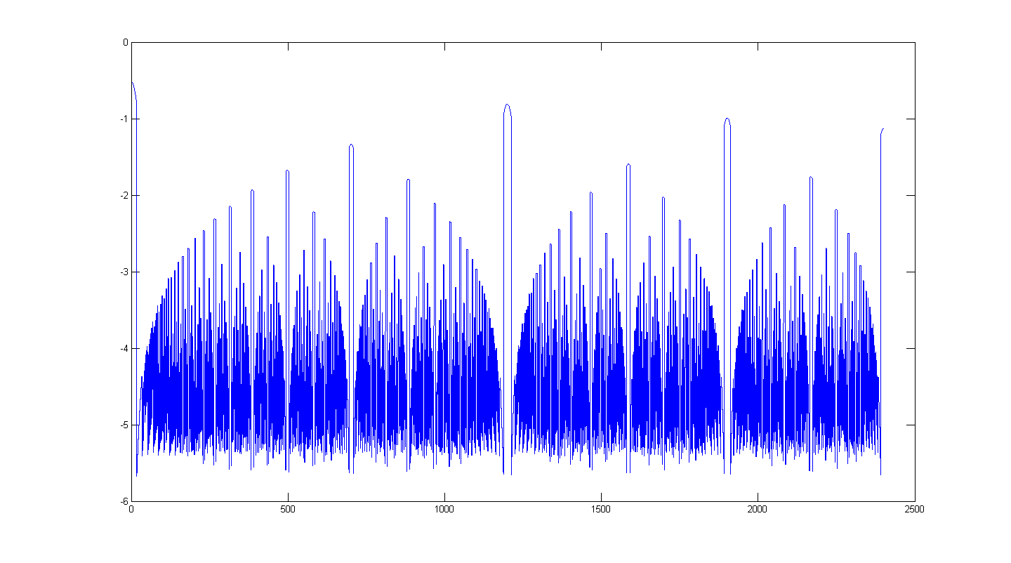
By convolving this with an upside-down Gaussian, HE is generated exactly:

(compare here: http://launch.groups.yahoo.com/group/harmonic_entropy/files/dyadic/default.gif)
In comparison, DC's basis function looks more like this:

It remains to be seen if the DC kernel can be scaled in such a way that the two converge for n*d<infinity. It is likely that both functions are related to Thomae's function, here:
http://en.wikipedia.org/wiki/Thomae%27s_function
And since Thomae's function is related to Euclid's orchard...
http://en.wikipedia.org/wiki/Euclid%27s_orchard
This could lead to some interesting psychoacoustic extensions to Tenney interval space.
Fast HE Algorithm
This is a work in progress - although this algorithm is mathematically sound, additional considerations need to be met to make this accurate in discrete-dyad space.So here's the fast HE algorithm in a nutshell:
1) Work out the widths for every interval - get mediant-to-mediant widths, or do sqrt(n*d), or whatever you want. The partitions can even overlap, but to make it like regular HE, make sure they don't overlap.
2) Construct the basis function K(d) - for every value d, figure out which partition K(d) lies in and compute log(C_s(i_u-d) - C_s(i_l-d)) at that point.
3) Convolve with a Gaussian.
As the Gaussian effectively lowpasses the signal, it might be possible to compute HE at a resolution of something like 20 cents, and use sinc interpolation to recover the curve at higher resolutions for a huge computational speedup and with minimal error.